Introduction

Tabular time series data with 590k train transactions and 500k test transactions.
443 columns as independent variables
“isFraud” is the dependent variable
Leader Board (LB) is based on the public and private AUC score.

Goal: Predict transactions that are isFraud==1.

Submission: CSV file with TransactionID and Probability of isFraud==1.

Grading: Based on AUC score.

Note: This is a year old competition that wont doesn’t allow “final submissions” anymore. Nevertheless I picked this competition to get experience in Tabular data, attempt my best solutions and learn from the greats.

Following is my systematic growth to a top 10% solution.

Columns explanation

TransactionDT: timedelta from a given reference datetime (not an actual timestamp)
TransactionAMT: transaction payment amount in USD
ProductCD: product code, the product for each transaction
card1 - card6: payment card information, such as card type, card category, issue bank, country, etc.
addr: address
dist: distance
P_ and (R__) emaildomain: purchaser and recipient email domain
C1-C14: counting, such as how many addresses are found to be associated with the payment card, etc. The actual meaning is masked.
D1-D15: timedelta, such as days between previous transaction, etc.
M1-M9: match, such as names on card and address, etc.
Vxxx: Vesta engineered rich features, including ranking, counting, and other entity relations.

Categorical Features:

ProductCD
card1 - card6
addr1, addr2
P_emaildomain
R_emaildomain
M1 - M9
id_12 - id_38

TL;DR

My final Kaggle Kernel is here:

The following are roughly the things that improved my score.

Method	Public LB	Private LB	Percentile
Baseline XGB	0.9384	0.9096	Top 90%
Remove 200 `V`	0.9377	0.9107	Top 80%
Remove time cols	0.9374	0.9109	Top 80%
Transform `D`	0.9429	0.9117	Top 50%
Combine cols and Frequency Encoding	0.9471	0.9146	Top 30%
Aggregation on uid1	0.9513	0.9203	Top 27%
Additional aggregations	0.9535	0.9220	Top 5%
Fillna	0.9537	0.9223	Top 5%
Changed UID	0.9543	0.9264	Top 2%

Main kernel of work done is here.

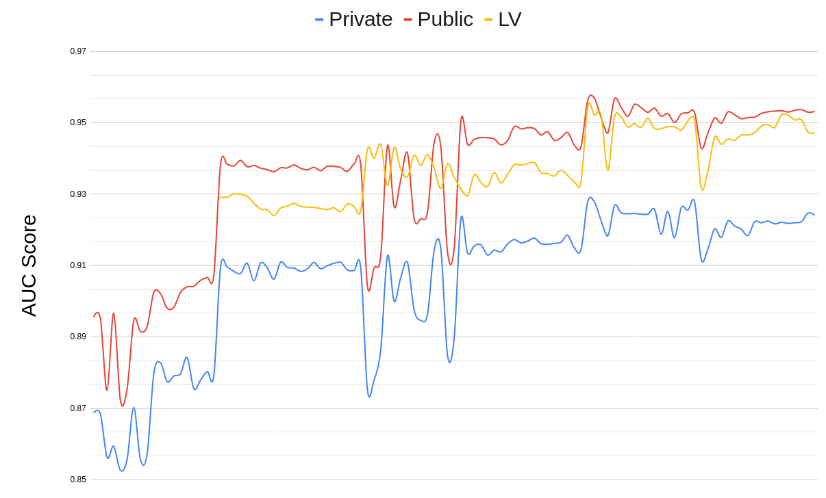
AUC score increase over time:

The Part that makes it hard to predict

We are not predicting Fraudulent Transactions. Once a client has a fraudulent transaction all the posterior transactions (associated with the useraccount, email address or billing address) are marked as fraud.

And it is not known as to What constitutes the client. Below is an example of an “assumed client-variable set”. Such a client could potentially have both isFraud=0 and isFraud=1 in their transactions, making it harder to detect clients with fraudulent transactions.

To make this even more difficult the meaning of most of the columns are obscured. For example, we know that D1 to D15 are some “timedeltas” such as days between each transaction, but don’t know what exactly they stand for. This goes for all 439 columns.

Way of work

Start with building a quick model after having a quick look at the data.
Do detailed EDA and test different ideas on the quick model.
submit model to get test score and iterate.

EDA

Lots of NaNs

The data has 254 variables (out of 439) with >25% NaNs.
I tried fillna, removing the columns completely and also just leaving them as NANs.
I found best results with filling NaNs with an artificial number such as -9999. Removing >25% NaN columns seems to remove critical information. Results with fillna were better by 0.0002 than leaving NaNs as it is.

Median Imputing doesn’t make sense

There are columns such as “card1” and “addr1” which denote credit card and address information respectively, but there is no way a median imputation makes any sense. So this is not done.

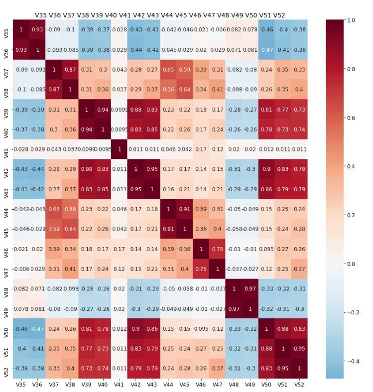
Reducing 339 `V` columns to 139 `V` columns

There were about 340 V columns said to be “engineered” by the company conducting the competition. They are engineered from the other 100 columns.

The V columns share a “lot” of correlation and a large number of Nan’s. The goal of this step is to find “similar” columns based on number of “NaN’s”, and Correlation>0.75. This process is automated for all the different NaN groups, using a script. The method is explained as below:

First group by NaN’s
Within each Nan group, highly correlated columns are binned together
The column with maximum unique values is chosen from each bin.

For example, V35 to V52 (17 columns) contain the exact same number of NaNs (168k). They contain 8 pairs of highly correlated columns as shown below. From this we select ['V36', 'V44', 'V39', 'V49', 'V47', 'V41', 'V40', 'V38'] (8 columns).

plt.figure(figsize=(15,15))
#mask = np.triu(xs_corr)
sns.heatmap(xs_corr, cmap='RdBu_r', annot=False, center=0.0)#, mask=mask)
plt.title('All Cols',fontsize=14)
plt.show()

Effect on LB and time: Small decrease in score for a large gain in computation time.

	public	private	time
baseline	0.9384	0.9096	11mins
remove 200 V columns	0.9377	0.9107	7mins

Reducing further

Tried reducing other columns, such as the C, M and ID columns in a same manner but then they reduced the LB by 0.01, so this is as far as the reduction goes.

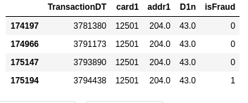
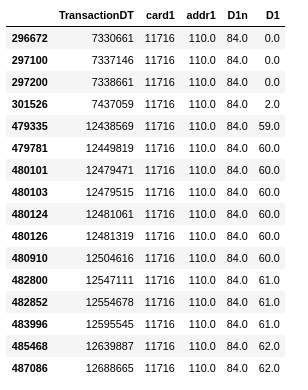
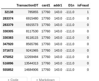
Understanding D columns

D1 column is known from the discussions to be “days since the client credit card began”. Subtracting this value from the “Transaction Day” will result in CONSTANT values per client. D1n is the created column after subtraction.

We do the same for all D columns irrespective, and allow the model to decide what is important and what is not. Following is an example of an “assumed client-variable set”. Notice how the D1n columns are constant and the D1 columns increase over time, when the data is sorted on TransactionDT.

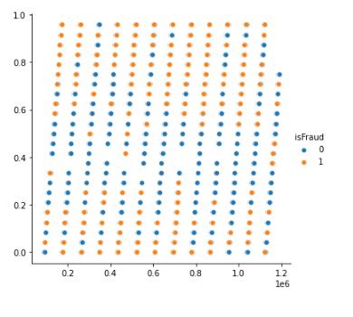
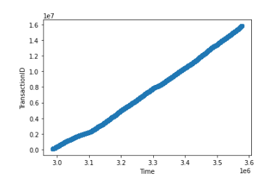
Another column D9 denotes the hours at which the transactions are done. This is tested using df["Hr"] = df["TransactionDT"]/(60*60)%24//1/24. The following plot clearly shows it’s relation to determining if a transaction is Fraud or not.

Unbalanced data

The Data has only 3.7% transactions denoted as “Fraud” (isFraud=1). RandomOverSampling and Smote didn’t do much for the score so I didn’t keep it.

EDA for UID

As said before this competition is not just about predicting fraudulent transactions over time, it’s about predicting clients who are more likely to have isFraud transactions. Client account, client email addresses and client address associated with a Fraudulent transactions is made isFraud==1 in a posterior fashion. We need to thus find these client variables (UIDs) to be able to predict better.

Finding the UIDs

I stood on the shoulders of giants, to find help on this part.

UIDs are nothing but variables that help identify a particular clients’ transactions. Not all transactions are fraud for a client but “most” are expected to be. This allows us to determine the quality of a UID.

To find the UID, a bit of guess and adversarial validation (AV) is used (AV is explained later). Based on how “isFraud” is defined we can already guess that card1, addr1 & P_emaildomain are probably part of UID. In addition we use AV to determine the rest of the columns.

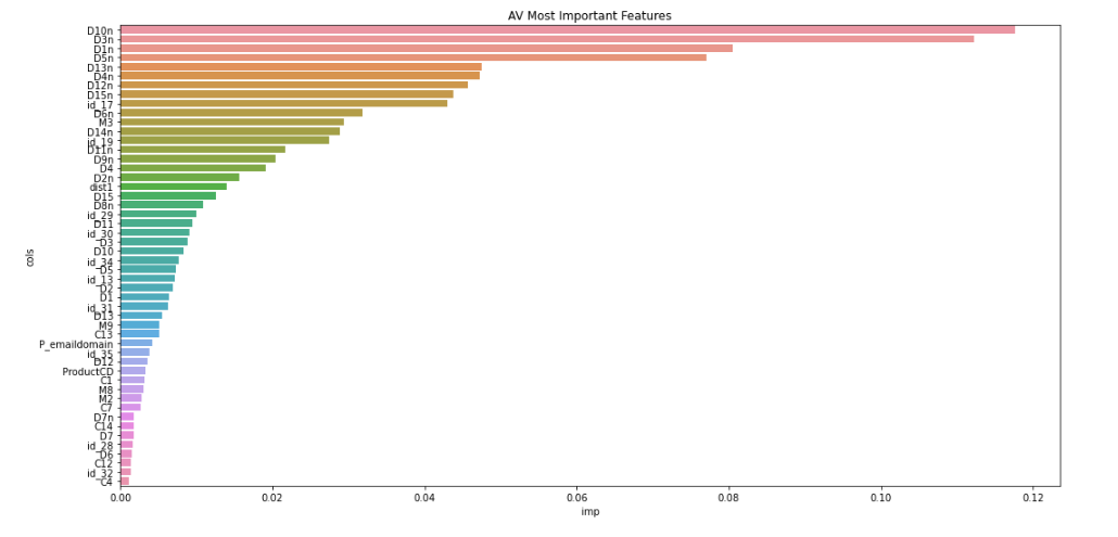
To evaluate how good the UID is, we look at how much percent of the clients have both isFraud==0 and isFraud==1 and we check manually if they happen one after the other in sequential manner. Shown below are the evaluations for different UIDs.

	Mixed	isFraud==1	isFraud==0
uid0	1.9%	1.9%	96%
uid1	1.4%	2.3%	96.3%
uid2	0.79%	2.6%	96.5%
uid3	0.43%	2.6%	96.9%
uid4	0.38	2.6%	97%

UID0: D10n, card1, addr1
UID1: D1n, card1, addr1
UID2: D1n,card1,addr1,p_emaildomain
UID3: D1n,card1,addr1,p_emaildomain, D3n
UID4: D1n,card1,addr1,p_emaildomain, D3n, V1, M7

In all cases “many” of the “Mixed” clients don’t have isFraud==0 and isFraud==1 sequentially (as shown below). So it looks like most of the Mixed clients are wrongly classified. I tried refining it with several other combinations but had little success. So I moved on to the testing out how these UIDs actually helped.

Final score with different UIDs (UID2 is the best)

	public LB		Private LB
uid1	0.9534	-	0.9220	-
uid2	0.954	+0.0006	0.925	+0.003
uid3	0.9464	-0.007	0.913	-0.012

Model

I started off with Random Forests, but didn’t get far with it. XGB, Catboost and LGBM seem to be preferred decision trees models in the ML community. So I chose XGB and stuck with it till the end to see what are the best results I can get with it. I used the default values and that was just good enough.

My classifier was made of:

    clf = xgb.XGBClassifier(n_estimators=2000, 
                        max_depth=8, 
                        learning_rate= 0.05,
                        subsample= 0.6,
                        colsample_bytree= 0.4, 
                        random_state = r.randint(0,9999),
                        use_label_encoder=False,
                        tree_method='gpu_hist')

As I wanted to get the max score possible, I used random_state = r.randint(0,9999), as this would not keep the random_state constant. Simulations in this manner produced variation in the order of +-0.002 AUC score in some cases. So when it is unclear if a hypothesis works or not, I run the same simulation a few times and take its average.

Ensembling is also an option but I haven’t tried it in this competition. Based on the top solutions they seem to improve the score too.

Feature engineering

Fillna

df.fillna(-9999,inplace=True)

XGB is capable of handling NaNs. It places the NaN rows in one of the splits at each node, (based on which gives a better impurity score). However if we choose a number to represent NaNs then it treats the NaNs like just another value/category. And it is a bit faster, due to lesser computations.

However fillna boosts the score only by 0.0002.
Label Encoding of Categorical data

All columns with <32000 unique values are made integers and label encoded. This is done to reduce the ram usage. A string in python uses almost twice as much memory as an integer. Label encoding is done using:

df.factorize()
One hot encoding the NaN structure for certain columns

D2 has 50% NaNs and is highly correlated (0.98) with D1. In this case D2 is removed and the NaN structure is alone kept.

D9 columns represents the time of transaction in a day. But it contains 86% NaN values. So a new D9 column (HrOfDay) was created from TransactionDT using df["Hr"] = df["TransactionDT"]/(60*60)%24//1/24. And the NaN structure of D9 is One Hot Encoded.
Splitting

There are many categorical columns, that would allow for better models when split. For example, we have “TransactionAmt”, which allows for the split: “dollars” and “cents”. cents could be a proxy for identifying if the transaction is from another country than US. Possibly there could be a pattern on how frauds happen with “cents”. The “split” is done using the following function:
```
 def split_cols(df, col):
 df['cents'] = df[col].mod(1)
 df[col] = df[col].floordiv(1)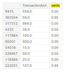
```
Another example is id_31. It has values such as chrome 65.0, chrome 66.0 for android. To aid the model we split the version number and browser using the commands below. The same has been done for several other columns, and kept if it resulted in an increase in score or featured high in the feature importance plots.
```
 lst_to_rep = [r"^.*chrome.*$",r"^.*aol.*$",r"^.*[Ff]irefox.*$"...]

 lst_val = ["chrome","aol","firefox","google","ie","safari","opera","samsung","edge","chrome"]
 df["id_31_browser"].replace(to_replace=lst_to_rep, value=lst_val, regex=True,inplace=True);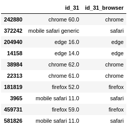
```
Combining

Combining values such as card1 and addr1, by themselves they might not mean much, but together they could correlate to something meaningful. One such combination is the UID. But we don’t keep the UID just as we don’t keep the time columns.
Frequency encoding

The frequency of the values of a column seems important to detect if a transaction is fraud or not.
```
 def encode_CB2(df1,uid):
     newcol = "_".join(uid)
     ## make combined column
     df1[newcol] = df1[uid].astype(str).apply(lambda x: '_'.join(x), axis=1)
```
Added several features based on this and resulted in increase in score (documented below).
Aggregation (transforms) while imputing NaNs

This is one of the most important parts of the solution which boosted the score all the way into top 10% from top 30%. Why Aggregations work is explained here. The aggregation is done after combining the train and test dataframes. The following groupby command does it all.

df_all.groupby(uid,dropna=False)["TransactionAmt"].transform("mean").reset_index(drop=True)

It is very important to add dropna=False, as there are many NaN rows which would be dropped otherwise. fillna is not done until the aggregations are made. This way, Nan’s in the aggregated column get imputed.

Finding the columns to be aggregated was possible using just the AV feature importance seen above and a bit of logic.
Removing redundant columns based on Feature Importance

As far as I have seen, removing redundant columns makes the model faster and rarely improves the score. Having said that I tried to remove columns that seemed redundant but got the score reduced by 0.002, which is a LOT in this competition. So I kept all those variables. However removing redundant V columns (200 of them) gives a large decrease in time of computation. So those are the ones that are removed.
Removing time columns such as TransactionDT and TransactionID

What worked and by how much

Method	Public LB		Private LB		Percentile
baseline	0.9384		0.9096		Top 80%
remove 200 `V`	0.9377	-0.003	0.9107	+0.001	Top 80%
remove time cols	0.9374	-0.0003	0.9109	+0.0002	Top 80%
Transform `D`	0.9429	+0.0055	0.9117	+0.0008	top 50%
Combine and FE	0.9471	+0.0042	0.9146	+0.0029	top 30%
Agg on uid1	0.9513	+0.0042	0.9203	+0.0057	top 20%
additional agg	0.9535	+0.0022	0.9220	+0.0017	top 10%
fillna	0.9537	+0.0002	0.9223	+0.0003	top 10%

Post Process

isFraud of the same clients are all expected to be 0 or 1. So, tried averaging the “identified-client’s” probabilities across train and test. This resulted in a poorer score by upto 0.003. So didn’t end up using it.

Local Validation and Prediction Strategy

Initially I started with a 10% sample dataset and looked at a hold out. Considering that it took 7 mins per simulation for the entire dataset, I went on to use the entire dataset instead of just the sample.

I tried a couple of strategies here and compared to test solution:

Holdout and predict average of 5 models
5Fold CV unshuffled.
Group 5fold CV based on Month

The following are the results:

	Local	Public LB	Private LB
5Fold CV unshuffled	baseline	baseline	baseline
Holdout (5x)	-0.01	-0.013	-0.016
Month 5fold CV	+0.0022	-0.0006	+0.0000

The Holdout method seems obviously not good. Month 5fold CV did not produce significant increases (>0.002) in LB so I skip it. All are compared to the baseline values (5fold CV unshuffled).

Note: As this is a time series simulation people had warned about not using CV: here, and here. However the best results, including that of the top solution for this competition were only possible due to CV.

Memory reduction

Label encoding of categorical variables.
Converting variables to float32 should be good enough.

16bit: 0.1235 32bit: 0.12345679 64bit: 0.12345678912121212

With the AUC numbers, 8 digits beyond the decimal seems good enough.
Removing 200 V columns out of the 439 columns with little change in score allowed to finally do AV on the kaggle kernel without going out of memory.

Practical understanding of Overfitting and AV

Preventing overfitting

There are usually two reasons why the Training score and Test score differ:

Overfitting
Out of Domain Data

i.e., test and train data are from different times, or different clients etc…

There is a nice trick to see what is causing the difference in scores between the training and the test data: Determining OOF (out-of-fold) scores. The OOF score is basically a score on unseen data but within the training data domain itself. It nicely controls for the effect of “out of domain” data. So,

OOF (out-of-fold) scores < Train scores ==> Overfitting
Test scores < OOF scores ==> Out-of-domain data

Example of only over-fitting

From the beginning I have suffered mainly with overfitting rather than the out-of-domain data issue. My OOF<<Train (indicating overfitting) and Test>OOF (not indicating “out-of-domain” issue):

	train	OOF	test (public)
baseline AUC	0.99	0.9292	0.9384

Example of both over-fitting and out of domain issue

In another case, where I accidentally changed some values of columns in the test dataset as NaNs, I saw the following. Here OOF<<Train (indicating overfitting) and also Test<<OOF (indicating “out-of-domain” issue):

	train	OOF	test (public)
AUC	0.9971	0.9426	0.9043

Looking at the important AV columns, and probing into those columns allowed me to fix the issue.

Preventing overfitting

What appears to reduce overfitting are:

removal of time and client columns such as TransactionID and TransactionDT, Created UIDs etc…
Other Feature Engineering based columns (Frequency Encoding, combining columns, and most important of all Aggregations).
Choosing the right parameters for the XGB model (i.e., depth of tree etc…).

What can your AV do for you?

Adverserial Validation is a simple technique that helps distinguish the difference in the train and the test data. In this kernel, I show how to do AV with a simple example. It involves the following steps:

Concat the train and the test data set.
Append a new column “is_test”.
Split data into training and validation.
Train model and get AUC score on istest==1 for the validating set.

AV can identify out-of-domain data

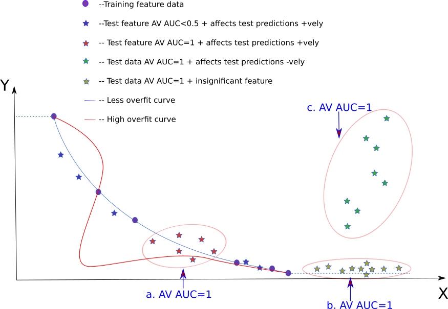
In the image above, the circles (blue) denote training data. The blue line denotes the line fit. Red line denotes an overfit line. Different colored stars (blue, green, red, yellow) denote different types of test data. Y is the dependent variable and X is the independent variable. The dotted blue line indicates the predicted value in case the data lies beyond the training bounds.

The three regions marked in “big bubbles” are where there is no training data and hence these are out-of-domain data regions. We simply get a very high AUC score (AUC=1) from AV for these (red, green and yellow stars). In this kernel it is checked with an example that the “big bubbles” in the image above have AV AUC=1.

AV AUC=1 and how they affect test predictions

When the test set is denoted by the green stars, it is clear that the resulting test score is going to be “bad”. However, when the test set is denoted by the yellow stars, error in predicting seems to be less in comparison (despite having AV AUC=1). When the test set is denoted by the red stars the error doesn’t seem to be that bad either AV AUC=1.

From the beginning to the end for this competition, I had >0.9 AUC, and nevertheless ended up with very good results (0.953–>top 10%). In addition the OOF score (from training) was less than the TEST score informing that the OUT-OF-DOMAIN data was not the problem for the score. I am thus inclined to think that in my case I probably end up with test data which are out of domain like the red and yellow stars and not like the green stars.

How AV is used in this kaggle competition

Identify and Remove time columns like TransactionID and TransactionDT

When AV is first run on this dataset, two columns standout: TransactionDT and TransactionID. One is the time info in seconds and the other is the id of each transaction. Ideally we don’t want to be using such time columns as we don’t want the model to learn anything specific to the Date or the ID of transactions. AV provides a platform to identify such variables and eventually we can get rid of them.
Removing very different columns for negligible score loss.

In one of the iterations I had 203 columns with an lb score of 0.953. Removing 20 of the most important AV columns resulted in a small decrease in score 0.9511. I always try to see how the “out of domain” data affects our result.
AV helps find aggregations that we need

This is and will be the greatest reason for doing AV. AV is so powerful that improving my score from top 80% to a top 10% score was done purely by looking at the important AV columns.

I pretty much used the first 10-20 important AV columns (and a few columns on my own) to determine which columns to choose as UID and which to aggregate over.

Find mistakes with your AV

I applied aggregation to the training dataset and accidentally did not apply it to the test. This was promptly visible in the AV as the aggregated columns showed up first in the “AV important columns”. A quick look at the top AV important columns and I found my error.

For example, in one of the experiments I got the following:

	train	OOF	test (public)
AUC	0.9971	0.9426	0.9043

From this it is possible to infer that there is both overfitting (train»OOF) and Out of Domain issue (OOF»test). Using AV, I was able to find out which columns were giving me the problem. When I probed in deeper into the columns, it turned out that I had accidentally added NaN’s to the test data.

Once I corrected for it, I ended up with:

	train	OOF	test (public)
AUC	0.998	0.9474	0.9530

Fraud Detection Tabular Kaggle competition

Introduction

Columns explanation

TL;DR

The Part that makes it hard to predict

Way of work

EDA

Lots of NaNs

Reducing 339 `V` columns to 139 `V` columns

Reducing further

Understanding D columns

Unbalanced data

EDA for UID

Model

Feature engineering

Post Process

Local Validation and Prediction Strategy

Memory reduction

Practical understanding of Overfitting and AV

Preventing overfitting

What can your AV do for you?

References

Introduction

Columns explanation

TL;DR

The Part that makes it hard to predict

Way of work

EDA

Lots of NaNs

Reducing 339 V columns to 139 V columns

Reducing further

Understanding D columns

Unbalanced data

EDA for UID

Model

Feature engineering

Post Process

Local Validation and Prediction Strategy

Memory reduction

Practical understanding of Overfitting and AV

Preventing overfitting

What can your AV do for you?

References

Reducing 339 `V` columns to 139 `V` columns