What worked and what didn’t work in my journey towards a top 10% score (standing on the shoulders of giants) in the fraud-detection-competition.

Feature engineering

Fillna

df.fillna(-9999,inplace=True)

XGB is capable of handling NaNs. It places the NaN rows in one of the splits at each node, (based on which gives a better impurity score). However if we choose a number to represent NaNs then it treats the NaNs like just another value/category. And it is a bit faster, due to lesser computations.

However fillna boosts the score only by 0.0002.
Label Encoding of Categorical data

All columns with <32000 unique values are made integers and label encoded. This is done to reduce the ram usage. A string in python uses almost twice as much memory as an integer. Label encoding is done using:

df.factorize()
One hot encoding the NaN structure for certain columns

D2 has 50% NaNs and is highly correlated (0.98) with D1. In this case D2 is removed and the NaN structure is alone kept.

D9 columns represents the time of transaction in a day. But it contains 86% NaN values. So a new D9 column (HrOfDay) was created from TransactionDT using df["Hr"] = df["TransactionDT"]/(60*60)%24//1/24. And the NaN structure of D9 is One Hot Encoded.
Splitting

There are many categorical columns, that would allow for better models when split. For example, we have “TransactionAmt”, which allows for the split: “dollars” and “cents”. cents could be a proxy for identifying if the transaction is from another country than US. Possibly there could be a pattern on how frauds happen with “cents”. The “split” is done using the following function:
```
 def split_cols(df, col):
 df['cents'] = df[col].mod(1)
 df[col] = df[col].floordiv(1)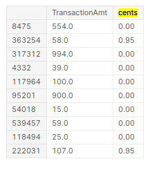
```
Another example is id_31. It has values such as chrome 65.0, chrome 66.0 for android. To aid the model we split the version number and browser using the commands below. The same has been done for several other columns, and kept if it resulted in an increase in score or featured high in the feature importance plots.
```
 lst_to_rep = [r"^.*chrome.*$",r"^.*aol.*$",r"^.*[Ff]irefox.*$"...]

 lst_val = ["chrome","aol","firefox","google","ie","safari","opera","samsung","edge","chrome"]
 df["id_31_browser"].replace(to_replace=lst_to_rep, value=lst_val, regex=True,inplace=True);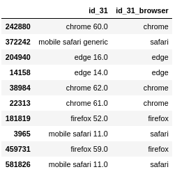
```
Combining

Combining values such as card1 and addr1, by themselves they might not mean much, but together they could correlate to something meaningful. One such combination is the UID. But we don’t keep the UID just as we don’t keep the time columns.
Frequency encoding

The frequency of the values of a column seems important to detect if a transaction is fraud or not.
```
 def encode_CB2(df1,uid):
     newcol = "_".join(uid)
     ## make combined column
     df1[newcol] = df1[uid].astype(str).apply(lambda x: '_'.join(x), axis=1)
```
Added several features based on this and resulted in increase in score (documented below).
Aggregation (transforms) while imputing NaNs

This is one of the most important parts of the solution which boosted the score all the way into top 10% from top 30%. Why Aggregations work is explained here. The aggregation is done after combining the train and test dataframes. The following groupby command does it all.

df_all.groupby(uid,dropna=False)["TransactionAmt"].transform("mean").reset_index(drop=True)

It is very important to add dropna=False, as there are many NaN rows which would be dropped otherwise. fillna is not done until the aggregations are made. This way, Nan’s in the aggregated column get imputed.

Finding the columns to be aggregated was possible using just the AV feature importance seen above and a bit of logic.
Removing redundant columns based on Feature Importance

As far as I have seen, removing redundant columns makes the model faster and rarely improves the score. Having said that I tried to remove columns that seemed redundant but got the score reduced by 0.002, which is a LOT in this competition. So I kept all those variables. However removing redundant V columns (200 of them) gives a large decrease in time of computation. So those are the ones that are removed.
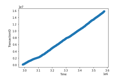
Removing time columns such as TransactionDT and TransactionID

What worked and by how much

Method	Public LB		Private LB		Percentile
baseline	0.9384		0.9096		Top 80%
remove 200 `V`	0.9377	-0.003	0.9107	+0.001	Top 80%
remove time cols	0.9374	-0.0003	0.9109	+0.0002	Top 80%
Transform `D`	0.9429	+0.0055	0.9117	+0.0008	top 50%
Combine and FE	0.9471	+0.0042	0.9146	+0.0029	top 30%
Agg on uid1	0.9513	+0.0042	0.9203	+0.0057	top 20%
additional agg	0.9535	+0.0022	0.9220	+0.0017	top 10%
fillna	0.9537	+0.0002	0.9223	+0.0003	top 10%

What worked and by how much--Feature engineering

Feature engineering

References